Project15 Jun 20215 min read

Computer vision projects

Classical computer vision projects covering filtering, features, clustering, eigenfaces, calibration, and homography.

A collection of classical computer vision projects from ENGN6528 Computer Vision at the Australian National University. The work spans low-level image processing, feature detection, unsupervised segmentation, face recognition, and projective geometry.

Source repository

Project Set#

The projects were implemented mostly in Jupyter notebooks using Python, NumPy, OpenCV, Matplotlib, and linear algebra routines from NumPy/SciPy. The point was to build the algorithms directly enough to understand the math, then compare the outputs against library implementations where appropriate.

The collection covers:

Area	Work
Image processing	colour channels, histograms, equalisation, filtering, translation, interpolation
Filtering	Gaussian smoothing and bilateral filtering in RGB and CIE-Lab colour spaces
Features	Harris corner detection from image gradients and corner response maps
Segmentation	KMeans and KMeans++ colour clustering
Recognition	Eigenfaces with PCA/SVD and nearest-neighbour matching
Geometry	camera calibration, intrinsic/extrinsic decomposition, homography estimation, image warping

Filtering and Colour Spaces#

The early image-processing work covered the basics: resizing, splitting RGB channels, computing histograms, applying histogram equalisation, converting RGB to YUV, and translating images with different interpolation strategies.

The more interesting part was denoising. Gaussian filtering smooths spatially nearby pixels, but it does not know whether a nearby pixel belongs to the same object or an edge across an object boundary. Bilateral filtering adds a second weighting term based on colour similarity, so pixels are weighted by both spatial distance and colour distance.

For a pixel $p$ , the bilateral filter can be written as:

I'(p) = \frac{1}{W_p} \sum_{q \in \Omega} I(q) \, G_{\sigma_s}(\lVert p - q \rVert) \, G_{\sigma_r}(\lVert I(p) - I(q) \rVert)

where $G_{\sigma_s}$ weights spatial distance, $G_{\sigma_r}$ weights colour/intensity distance, and $W_p$ normalizes the result.

The report compared RGB and CIE-Lab filtering. The reason CIE-Lab matters is that Euclidean distance in RGB is not perceptually uniform: two colours can be numerically close while looking different, or numerically far while looking similar. CIE-Lab gives the colour-distance term a better relationship to human perception.

Harris Corners#

The Harris corner detector was implemented from the image gradients up:

Convolve the image with derivative filters to obtain $I_x$ and $I_y$ .
Smooth products of derivatives with a Gaussian window.
Build a local second-moment matrix.
Compute the corner response:

R = \det(M) - k \operatorname{trace}(M)^2

Apply non-maximum suppression and thresholding.

Harris corner detection result

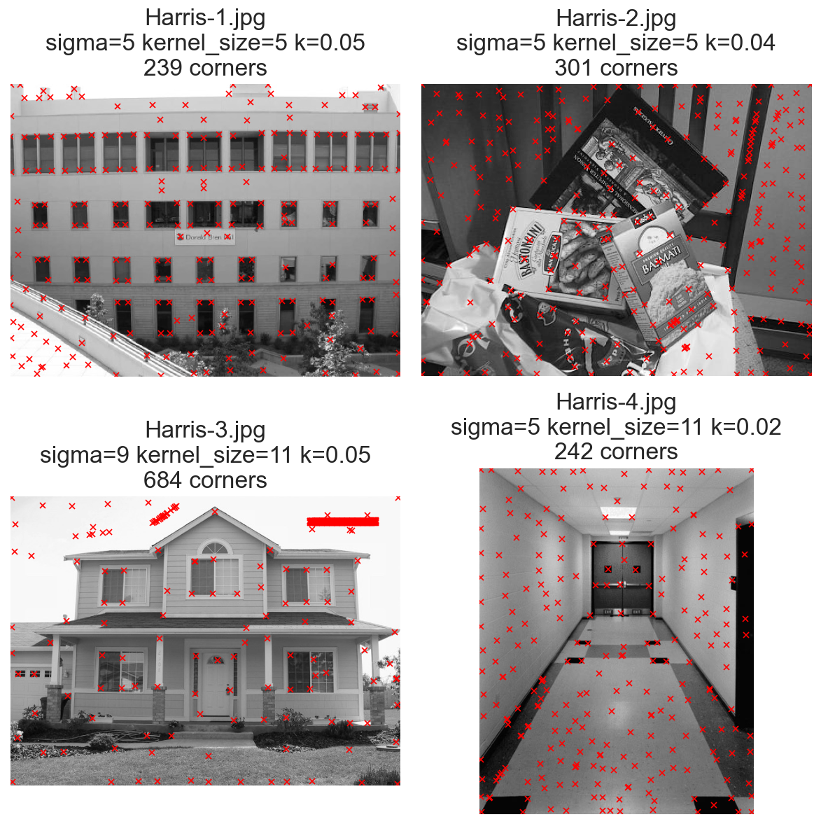
The useful lesson was not just detecting corners, but understanding when the detector fails. On images with no true two-directional intensity structure, the response map stays near zero except at artificial boundaries introduced by padding or image borders. Harris is translation-invariant, but it is not scale-invariant; smoothing scale, derivative masks, neighbourhood size, and the $k$ parameter all affect the result.

KMeans Segmentation#

The segmentation project implemented naive KMeans and KMeans++ for image clustering. Pixels were represented in colour space, with experiments that either included or excluded pixel coordinates.

KMeans minimizes within-cluster squared distance:

\sum_{i=1}^{n} \min_{j \in \{1,\dots,k\}} \lVert x_i - \mu_j \rVert^2

The KMeans++ version changed only initialization: instead of choosing initial centroids uniformly at random, it chose new centroids far from the nearest existing centroid. That made convergence less dependent on unlucky starting points.

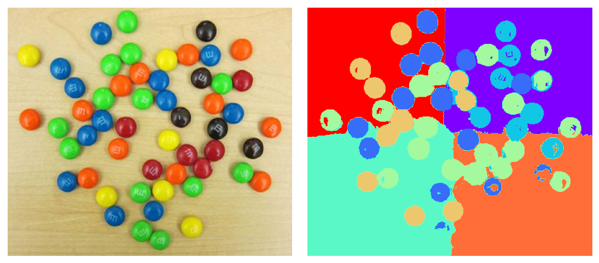
KMeans++ colour clustering on an M&M image

One practical observation was that including pixel coordinates can hurt object-level segmentation. It encourages the model to split an otherwise consistent background into spatial blocks, because nearby pixels become artificially more similar than visually similar pixels in different parts of the image. For this task, clustering on colour without coordinates produced cleaner object groups.

Eigenfaces#

The face-recognition project used PCA to build an Eigenface representation. Each aligned face image was flattened into a vector, centered by subtracting the mean face, then projected into a lower-dimensional face space.

The core decomposition was:

X \approx U_k \Sigma_k V_k^\top

where $k$ controls how many principal components are kept.

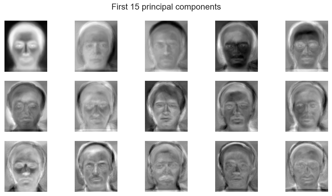
Top eigenfaces from the PCA face model

Alignment matters because Eigenfaces are not invariant to position or scale. A face image is treated as a vector where each pixel coordinate is a feature. If the eyes, nose, and mouth move around between images, PCA spends capacity explaining translation and scale artifacts instead of identity-relevant variation.

The report used SVD directly rather than eigendecomposing the full pixel covariance matrix. That is much cheaper because the number of images is far smaller than the number of pixels. The projected test images were then classified with nearest-neighbour search in face space.

Camera Calibration#

The geometry project estimated a camera projection matrix from 3D world points and 2D image correspondences using Direct Linear Transformation.

The camera model is:

\tilde{x} = P \tilde{X}

where $\tilde{X}$ is a homogeneous 3D world point, $\tilde{x}$ is a homogeneous image point, and $P$ is the $3 \times 4$ camera projection matrix.

The estimated matrix in the report was:

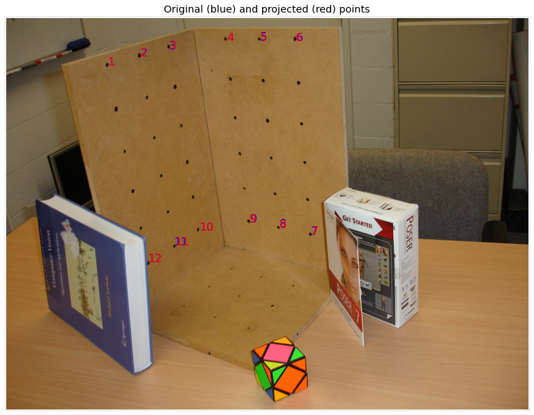
P = \begin{bmatrix} 0.0089 & -0.0041 & -0.0133 & 0.6928 \\ -0.0004 & -0.0156 & 0.0023 & 0.7208 \\ 0 & 0 & 0 & 0.0021 \end{bmatrix}

Projected calibration points after estimating the camera matrix

The reprojection mean squared error was about $0.5426$ pixels on the selected correspondences. The project then decomposed $P$ into intrinsic and extrinsic parameters:

P = K [R \mid t]

with focal lengths around $f_x = 908.78$ pixels and $f_y = 892.36$ pixels. Resizing the image roughly halved the focal lengths and principal point coordinates, while the rotation stayed approximately unchanged, which matches the geometry.

Homography and Warping#

The final piece estimated a two-view planar homography. Given corresponding points between two images, the project solved for:

\tilde{x}' = H \tilde{x}

using a Direct Linear Transformation system built from manually selected correspondences.

The estimated homography was:

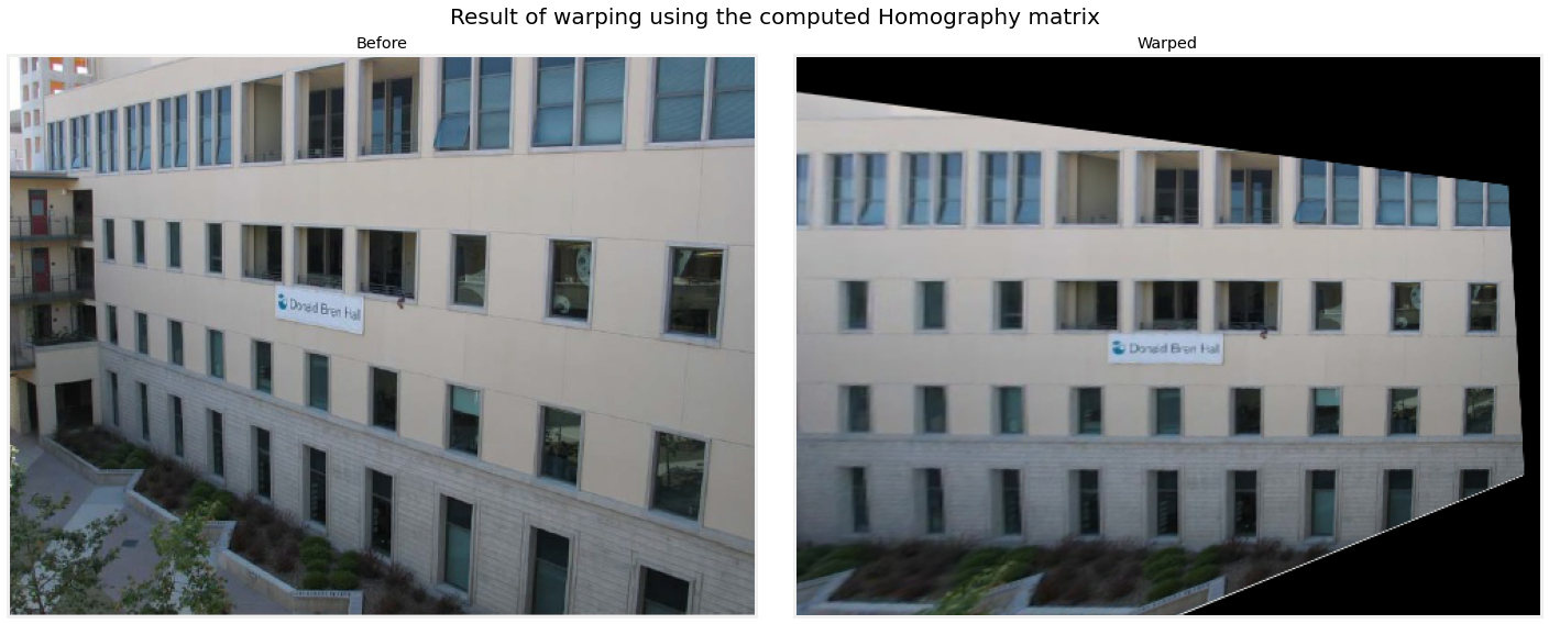
H = \begin{bmatrix} -0.0149 & 0.0004 & 0.9997 \\ -0.0024 & -0.0065 & 0.0169 \\ 0 & 0 & -0.0047 \end{bmatrix}

Image warped with the estimated homography

After warping, the point-transfer error was small: the report measured per-point distances under roughly one pixel for most selected correspondences and a mean squared error of about $0.3556$ pixels. The remaining error mostly came from manual point selection.

Reflection#

This was a useful pass through the classical computer vision stack. The algorithms are old, but they make the assumptions visible:

Harris corners depend on local gradient structure and scale.
KMeans segmentation depends heavily on the feature representation.
Eigenfaces work only when alignment makes pixel coordinates comparable.
Calibration and homography are linear algebra problems, but correspondence quality dominates the result.

The common thread is that computer vision models are often less about the final formula than about the representation you feed into it: colour space, coordinate system, scale, alignment, and correspondences all decide what the algorithm is allowed to see.