6 min read1,371 words
Transfer entropy across financial markets
A transfer-entropy study of directional information flow across market indices and industry ETFs.
A research project for CSYS5030 Information Theory and Self-Organisation at the University of Sydney. I used transfer entropy to ask a narrow question about financial time series: can we estimate the direction of information flow between economies and industries, rather than only measuring whether their returns move together?
Motivation#
The headline hypothesis was that the United States market, represented by the S&P 500, has more influence on the Japanese market, represented by the Nikkei 225, than Japan has on the United States.
That is not a question correlation can answer. Correlation is symmetric:
Mutual information measures how much knowing one variable reduces uncertainty about another; if two variables are independent, their mutual information is zero:
It is also symmetric. Correlation and mutual information can both tell you that two processes share information, but neither tells you whether the past of improves prediction of future more than the past of improves prediction of future .
Transfer entropy is asymmetric, so it is a better fit for that question. In this project I treated it as a measure of directed predictive information, not as proof of economic causality.
Dataset#
The report used daily Yahoo Finance data for three groups:
| Group | Instruments |
|---|---|
| Market indices | S&P 500 (^GSPC), Euronext 100 (^N100), Nikkei 225 (^N225), Bovespa (^BVSP) |
| Industry ETFs | Oil (USO), clean energy (ICLN), airlines (JETS), transportation (IYT), consumer staples (XLP), semiconductors (SMH), telecom (IXP), technology (VGT), pharmaceuticals (XPH) |
| Company stocks | ExxonMobil (XOM) and Delta Air Lines (DAL) |
The market indices were denominated in local currencies, but the analysis did not compare raw prices directly. Each adjusted close series was converted into log daily return:
This was a necessary preprocessing step. Price levels are not stationary and are not meaningfully comparable across markets: the fact that one index has a larger nominal value than another says little about its influence. Log returns move the analysis from price level to day-to-day movement.
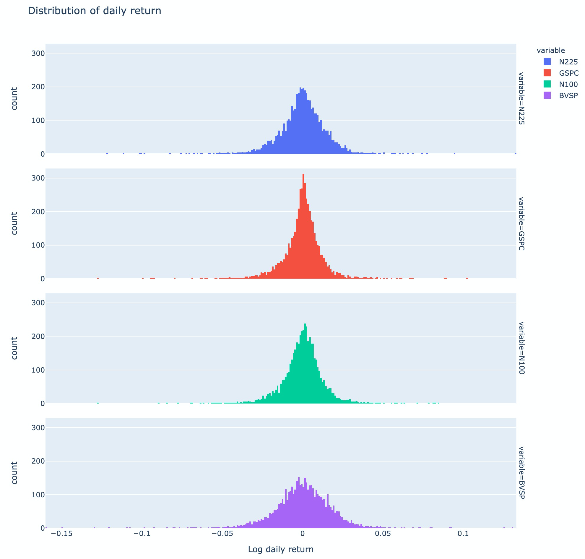
The return distributions were roughly symmetric but had different tail behavior. Brazil, treated in the report as an emerging-market proxy, showed heavier tails than the developed-market indices.
Method: Transfer Entropy#
Transfer entropy measures how much information from the source process helps predict the next state of the destination process, after accounting for the destination's own history.
For source and destination , the report used:
The directional comparison was then expressed as net information flow:
If , then the source carries more predictive information about than carries about , under the estimator and sampling window used.
Implementation#
The notebook wrapped the Java Information Dynamics Toolkit through jpype and used TransferEntropyCalculatorKraskov. The Kraskov estimator was chosen because the variables are continuous; a discretized estimator would require arbitrary bin choices, and a Gaussian estimator would focus on linear structure.
The main transfer-entropy settings were:
| Parameter | Value |
|---|---|
| History length | |
| Nearest neighbours | |
| Units | nats, using natural logarithms |
| Significance samples | 100 surrogate samples for selected all-period tests |
The notebook also used a k-nearest-neighbour Shannon entropy estimator from NPEET for exploratory entropy checks. For matrix-style summaries, small negative transfer-entropy estimates were clamped to zero before contribution totals were computed.
Market Results#
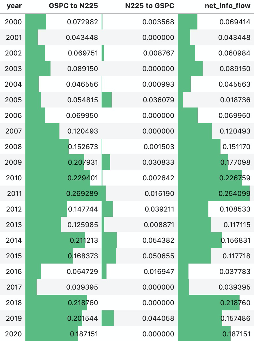
The S&P 500 to Nikkei 225 direction was larger than the reverse direction in every yearly window from 2000 to 2020.
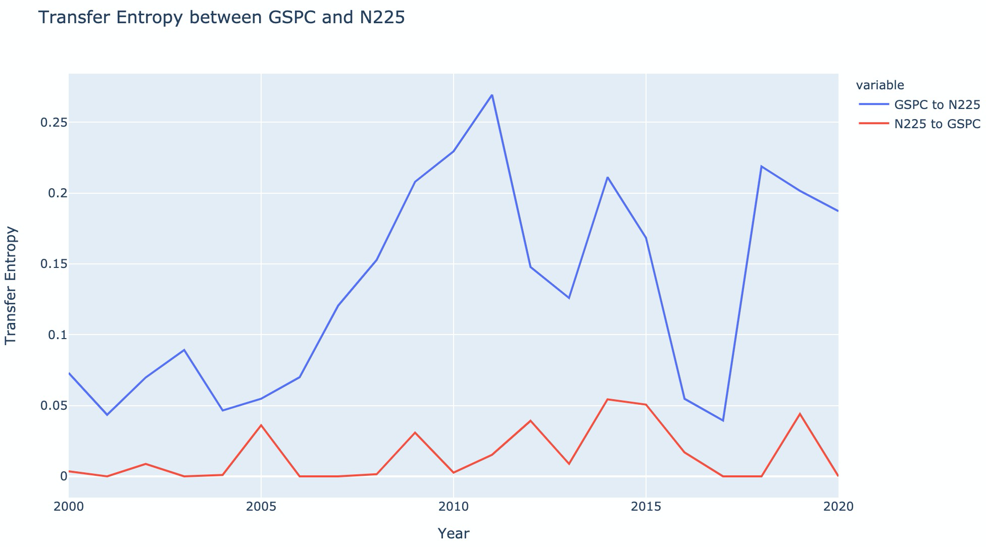
The yearly net flow was positive throughout the tested period:
Across the full 2000-2020 period, the all-period test produced:
| Direction | Transfer entropy | Significance |
|---|---|---|
| S&P 500 Nikkei 225 | nats | |
| Nikkei 225 S&P 500 | nats | |
| Net S&P 500 Nikkei 225 | nats | Positive |
The result supports the original hypothesis: in this dataset, U.S. market returns carried substantially more predictive information about Japanese market returns than the reverse.
The broader four-market transfer-entropy matrix showed a similar pattern.
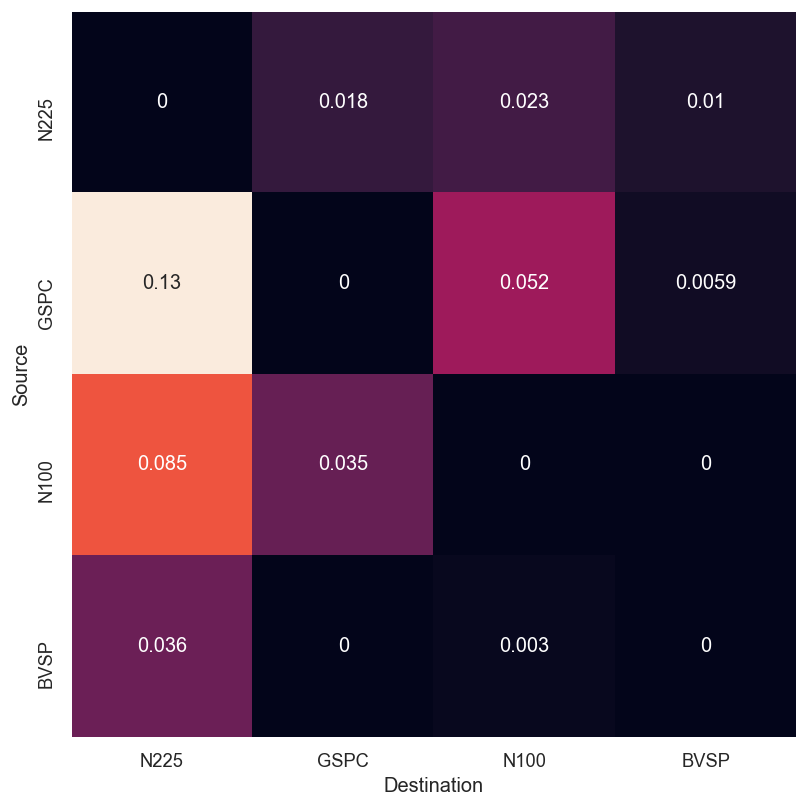
After summing outgoing transfer entropy by source and normalizing, the source contributions were:
| Source index | Normalized contribution |
|---|---|
| S&P 500, United States | |
| Euronext 100, Europe | |
| Nikkei 225, Japan | |
| Bovespa, Brazil |
The U.S. contribution was nearly as large as Europe, Japan, and Brazil combined. One interesting exception in the report was Japan versus Brazil: the Japan-to-Brazil direction was larger than Brazil-to-Japan, but the test was not statistically significant under the selected settings.
Industry Results#
The second half of the project applied the same idea to industry-sector ETFs. This made the analysis more speculative, because ETFs are imperfect industry proxies: they can be diversified, overlap in holdings, and start trading at different dates.
The notebook handled this in two ways. For pairwise ETF transfer entropy, it used the overlapping history available for each pair. For the common-window comparison, it used the longest shared ETF window in the dataset, beginning around May 2015 and ending in October 2020.
The yearly contribution chart highlighted which sector ETF had the largest share of outgoing transfer entropy in each year.
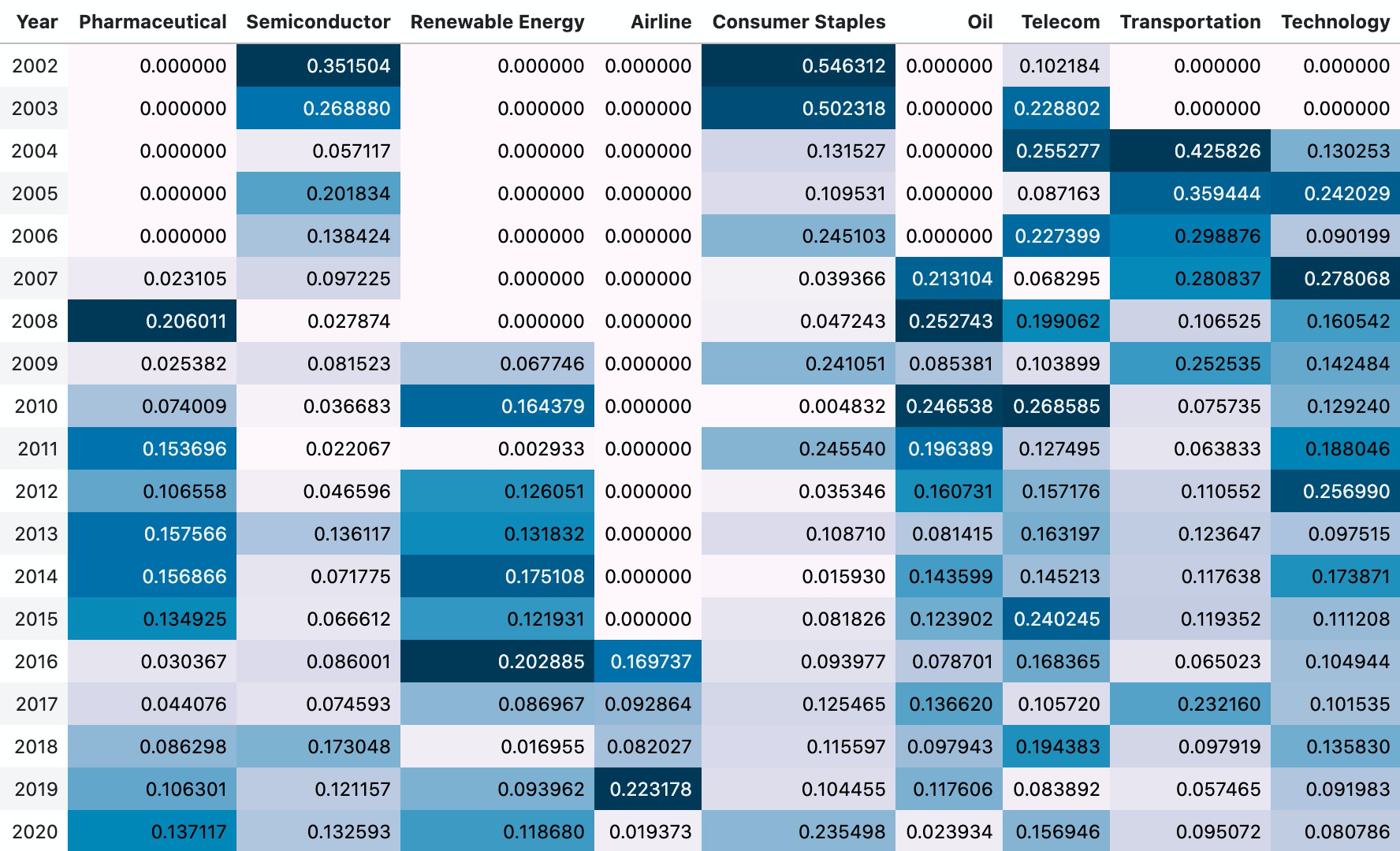
The report used a few historical examples to sanity-check the chart rather than claiming a trading model:
- Pharmaceuticals, 2007-2008: the report connected elevated pharmaceutical-sector contribution to a period of major genome-sequencing cost reductions.
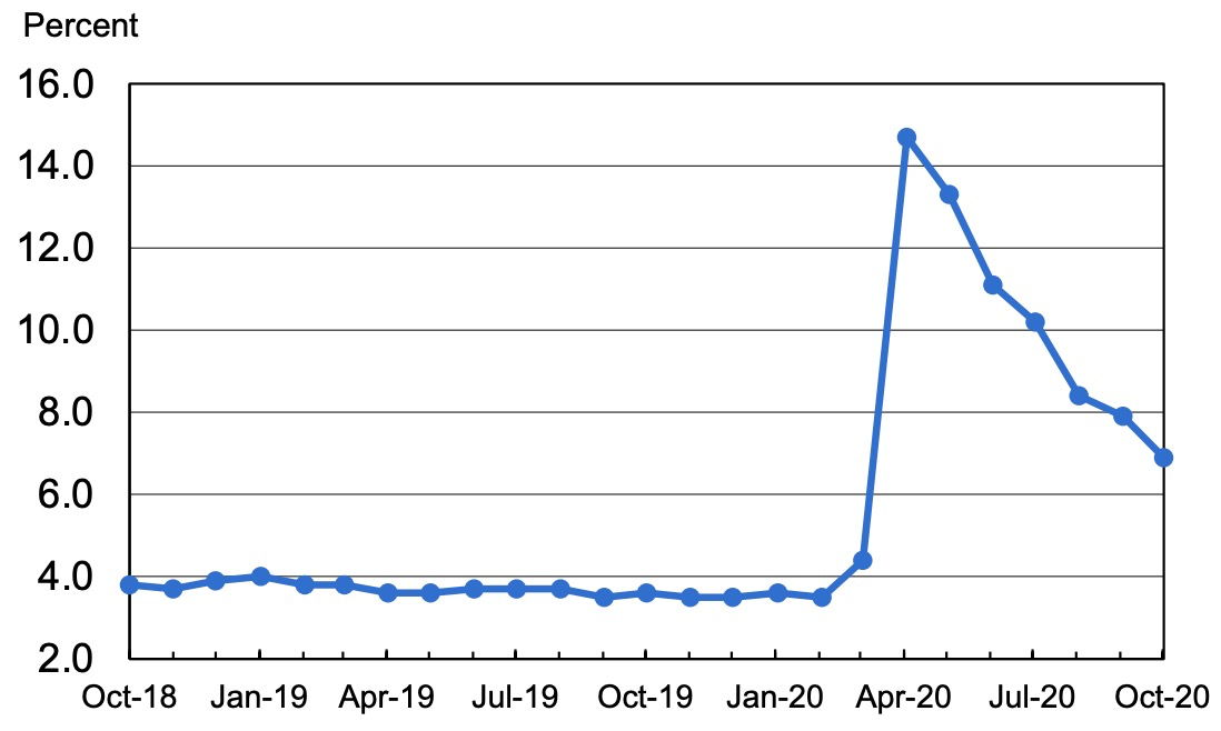
- Consumer staples, 2020: consumer staples became more prominent during the COVID-19 shock, consistent with the sector's defensive behavior during economic downturns.
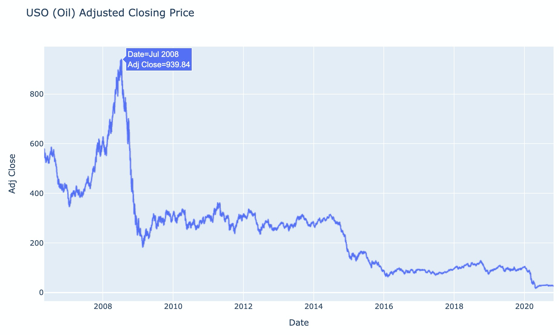
- Oil, 2008: oil showed a large event-driven move around the financial crisis and crude-oil price crash.
The interesting part here was not that every highlighted sector had a clean causal story. It was that transfer entropy produced a different kind of map from correlation: it emphasized which series were most informative as sources, not simply which series moved together.
Limits#
The strongest limitation is proxy quality. Market indices are reasonable economy-level summaries, but ETFs are messy industry summaries. If two sector ETFs hold overlapping companies, transfer entropy can reflect shared constituents rather than information transfer between industries.
The second limitation is estimator sensitivity. The project used and , which were reasonable for the sample size, but different history lengths, nearest-neighbour counts, or sampling windows could change the magnitude of the estimates.
The third limitation is interpretation. Transfer entropy is directional, but directionality is not the same as causality. A third process can drive both and , and market closing times, holidays, timezone differences, and asynchronous trading can all affect measured predictability.
Reflection#
I would keep the core structure: transform prices into returns, estimate and , then summarize net information flow. The parts I would rebuild are mostly experimental design.
For the industry analysis, I would replace ETFs with explicitly constructed baskets of stocks where each company belongs to one sector only. That would reduce overlap and make sector-to-sector transfer entropy easier to interpret.
I would also make uncertainty a first-class output. The original report includes significance checks for the headline market comparison, but a stronger version would show permutation-test distributions or confidence intervals for every matrix cell, then report sensitivity across , , and window length.
Finally, I would separate three claims that the first version blended together: predictive information, market influence, and economic causality. Transfer entropy can speak directly to the first, suggest the second, and only weakly gesture at the third without a stronger causal design.